
mlframe


A machine-learning framework for tabular data with a single entry point,
train_mlframe_models_suite, that trains, evaluates, calibrates, ensembles, and
reports across scikit-learn, CatBoost, LightGBM, XGBoost, HistGradientBoosting,
and PyTorch Lightning models on one dataset. It handles polars and pandas frames,
mixed dtypes, text features, ranking and quantile targets, and composite-target
stacking through a uniform API.
The changelog lives in CHANGELOG.md. Full guide index, including baseline diagnostics, honest-diagnostics, calibration policy, composite-target config reference, and error-decoding guides: docs/README.md.
Installation
mlframe depends on pyutilz, a sibling
utility library (parallel execution, pandas/polars helpers, hardware
introspection). Neither package is published to PyPI yet, so install both from
source — pyutilz first, then mlframe:
git clone https://github.com/fingoldo/pyutilz.git
git clone https://github.com/fingoldo/mlframe.git

pip install -e ./pyutilz
pip install -e ./mlframe
The core install pulls a compact stack (numpy, pandas, polars, scipy, scikit-learn,
pyarrow, joblib, tqdm, pydantic, numba), plus matplotlib and several other packages
that are imported unconditionally at module load time -- see pyproject.toml's
[project.dependencies] for the exact list. Heavier stacks ship as optional extras:
pip install mlframe[all,dev]                     # full install (recommended)

pip install -e "./mlframe[boosting]"             # catboost + lightgbm + xgboost
pip install -e "./mlframe[calibration]"          # shap + venn-abers + netcal + betacal + pycalib
pip install -e "./mlframe[neural]"               # torch + lightning + captum + transformers
pip install -e "./mlframe[automl]"               # flaml (HPO)
pip install -e "./mlframe[feature_engineering]"  # pysr (symbolic regression) + optbinning
pip install -e "./mlframe[sampling]"             # imbalanced-learn + iterative-stratification
pip install -e "./mlframe[polars_ext]"           # polars-talib + polars-ds
pip install -e "./mlframe[viz]"                  # matplotlib + plotly + seaborn + altair + hvplot
pip install -e "./mlframe[mlflow]"               # mlflow experiment tracking
pip install -e "./mlframe[db]"                   # sqlalchemy + psycopg2 + duckdb + pymongo + zstandard
pip install -e "./mlframe[signal]"               # antropy + astropy + pywavelets + ruptures
pip install -e "./mlframe[unsupervised]"         # hdbscan + umap-learn
pip install -e "./mlframe[stats]"                # statsmodels
pip install -e "./mlframe[gpu,transformer_gpu]"  # cupy + gpu-info + cupy-cuda12x for the GPU stages (match your CUDA build)
pip install -e "./mlframe[transformer,transformer_ann]"  # transformer-style FE (numba-only CPU path) + hnswlib for approximate-NN at N >= 500k
pip install -e "./mlframe[all]"                  # runtime extras EXCEPT the CUDA-build-specific gpu / transformer_gpu (install those explicitly on a CUDA host)
pip install -e "./mlframe[dev]"                  # pytest + coverage + ruff + black + mypy + bandit + pre-commit
Requires Python 3.9 or newer; tested on 3.9 through 3.14. The full core stack
(numpy, numba/llvmlite, polars, scikit-learn, pyarrow, pydantic) ships cp314
wheels and the numba JIT kernels compile and run on 3.14.
For development:
git clone https://github.com/fingoldo/mlframe.git
cd mlframe
pip install -e ".[all,dev]"
pre-commit install
pytest
Modules
| Sub-package | Purpose |
|---|---|
mlframe.training | End-to-end training pipeline: train_mlframe_models_suite, per-model strategies, configs, feature handling, dummy baselines, AutoML, neural nets |
mlframe.feature_engineering | Numerical / time-series / financial / categorical / Hurst / MPS features, brute-force PySR search |
mlframe.feature_selection | MRMR (multiple variants), RFECV, Boruta-SHAP, mutual-information and optbinning filters and wrappers |
mlframe.metrics | Calibration (ICE, ECE, Brier REL/RES/UNC, CMAEW), classification (KS, MCC, Cohen kappa, balanced accuracy, G-mean, BSS, Gini, F-beta, Lift@k, Hosmer-Lemeshow, top-k, RPS), regression (RMSLE, MAPE/SMAPE/MASE, MBE, NSE, Poisson/Gamma/Tweedie deviance, rank correlations), multilabel and LTR metrics, CRPS-from-quantiles, drift (PSI/KL/JS/Wasserstein), and plotting |
mlframe.evaluation | Performance reporting across CV folds and holdout sets |
mlframe.calibration | Calibration diagnostics and isotonic / Platt / beta / Venn-Abers post-hoc calibrators |
mlframe.models | Ensembling (stack / blend / vote), hyperparameter optimisation, splitting strategies |
mlframe.estimators | scikit-learn-compatible custom estimators, early-stopping-aware wrappers, pipelines |
mlframe.preprocessing | NaN cleaning, scaling, outlier handling, clustering |
mlframe.inference | Batch and streaming prediction, SHAP / permutation explainability |
mlframe.reporting | Matplotlib and plotly chart backends, spec-driven panel rendering |
mlframe.core | numba-accelerated array ops, statistical helpers, EWMA, spectral matrix seriation, robust location estimators |
mlframe.data | Built-in and synthetic dataset generators |
mlframe.testing | Parametric frame generation for property-based tests |
mlframe.integrations | Optional third-party integrations (MLflow) |
mlframe.utils | EDA, experiments, text, ParamOracle data-dependent parameter learning, and miscellaneous helpers |
mlframe.inspection | Model-agnostic interpretation primitives absent from sklearn.inspection (Friedman-Popescu H-statistic interaction detection) |
mlframe.signal | DTW alignment and Gaussian-Process smoothing/confidence features for irregularly-sampled series |
mlframe.system | GPU import guards and kernel-tuning-cache integration shared across subpackages |
mlframe.votenrank | Ensemble-blending strategies beyond mlframe.models (confidence-gated, adversarial-stochastic, rank-splice, KNN-fallback blends) |
mlframe.competition | Kaggle-only exploratory tricks (data de-anonymization, leak exploitation); not for production, never imported by mlframe itself |
mlframe.data_valuation | Per-row Shapley/Banzhaf data valuation (KNN-Shapley, TMC-Shapley) for label-noise detection and sample-weighting |
Quick examples
One-call multi-model training and evaluation. Each model is trained with its
native preprocessing strategy (CatBoost / LightGBM / XGBoost on raw frames; linear
and neural pipelines get encoded, imputed, and scaled). The suite returns a
(models, metadata) tuple: models is a per-target-type dict of trained model
entries, metadata carries fit-time metrics, calibration diagnostics, baseline
diagnostics, and the reporting spec. The features and targets are pulled from the
frame by a caller-supplied extractor (see SimpleFeaturesAndTargetsExtractor).
import numpy as np, pandas as pd
from mlframe.training.core import train_mlframe_models_suite
from mlframe.training.extractors import SimpleFeaturesAndTargetsExtractor

rng = np.random.default_rng(0)
df = pd.DataFrame({"x1": rng.normal(size=500), "x2": rng.normal(size=500), "x3": rng.integers(0, 5, size=500)})
df["y"] = df["x1"] * 2 - df["x2"] + rng.normal(scale=0.1, size=500)
X_new = df[["x1", "x2", "x3"]].iloc[:5]

fte = SimpleFeaturesAndTargetsExtractor(regression_targets=["y"])

models, metadata = train_mlframe_models_suite(
    df=df,
    target_name="y",
    model_name="exp_quickstart",
    features_and_targets_extractor=fte,
    mlframe_models=["lgb"],
)

# `models` is keyed by target-type, then target name; the value is a list with one
# entry per requested model (plus ensembles, if enabled), each exposing the fitted model.
entry = models["regression"]["y"][0]
y_pred = entry.model.predict(X_new)

# Diagnostics live in `metadata` (per target-type, per target).
print(metadata["baseline_diagnostics"]["regression"]["y"])
Composite-target regression. A scikit-learn-compatible wrapper that fits a
single inner regressor on a transformed target (e.g. T = y - alpha*base) and
inverts the transform at predict time, exposing residual structure the raw target
buries. Pick the transform by name (list_transforms() enumerates them) and name
the base-feature column it residualises against. The wrapper clones the inner
estimator, delegates feature_importances_ / get_booster() / other attributes
transparently, and pins cross-version behaviour in CI.
import numpy as np, pandas as pd
from sklearn.ensemble import RandomForestRegressor
from mlframe.training.composite import CompositeTargetEstimator

rng = np.random.default_rng(0)
y_prev = rng.normal(size=300)
X_train = pd.DataFrame({"y_prev": y_prev, "x1": rng.normal(size=300)})
y_train = y_prev + X_train["x1"] * 0.5 + rng.normal(scale=0.1, size=300)
X_new = X_train.iloc[:5]

est = CompositeTargetEstimator(
    base_estimator=RandomForestRegressor(),
    transform_name="linear_residual",
    base_column="y_prev",
)
est.fit(X_train, y_train)
est.predict(X_new)
est.feature_importances_       # delegated from the fitted inner estimator
The wrapper above is the manual entry point. train_mlframe_models_suite also runs automatic composite-target discovery (CompositeTargetDiscovery / CompositeTargetDiscoveryConfig), which screens transforms, ensembles the survivors, and caches results; set MLFRAME_DISABLE_COMPOSITE=1 to turn it off. See docs/examples/composite_targets.md and the tutorial notebook.
Per-target metric panel. fast_calibration_report computes the Brier
reliability / resolution / uncertainty decomposition, ICE bands, ECE, ROC/PR AUC,
and the classification scores in one numba-accelerated pass, returning them as a
CalibrationReport NamedTuple (and, optionally, the calibration figure). The
result unpacks positionally and indexes exactly like the historical flat tuple, and
also exposes every element as a named attribute (report.brier_loss, report.ece, ...).
from mlframe.metrics import fast_calibration_report

# Positional unpacking still works (back-compatible with the flat 17-tuple):
(brier_loss, cal_mae, cal_std, cal_coverage,
 ece, brier_rel, brier_res, brier_unc,
 roc_auc, pr_auc, ice, ll, precision, recall, f1,
 metrics_string, fig) = fast_calibration_report(
    y_true=y_test,
    y_pred=clf.predict_proba(X_test)[:, 1],
    nbins=15,
    show_plots=False,
)
print(brier_rel, brier_res, brier_unc, ece)

# Or keep the result and use named access (clearer, index-safe):
report = fast_calibration_report(
    y_true=y_test,
    y_pred=clf.predict_proba(X_test)[:, 1],
    nbins=15,
    show_plots=False,
)
print(report.brier_reliability, report.brier_resolution, report.ece, report.roc_auc)
print(report[0] == report.brier_loss)  # True — positional indexing preserved
MRMR / RFECV feature selection. Several MRMR variants (FCQ, MID, FCD, plus
n-way interaction extensions) and an RFECV wrapper that reads LightGBM / XGBoost /
CatBoost feature importances correctly. Both are scikit-learn fit / transform
estimators; the selected columns land on the fitted estimator after fit(X, y).
import numpy as np, pandas as pd
from lightgbm import LGBMClassifier
from mlframe.feature_selection.filters.mrmr import MRMR
from mlframe.feature_selection.wrappers import RFECV

# X, y are reused by every snippet below in this section.
rng = np.random.default_rng(0)
X = pd.DataFrame(rng.normal(size=(400, 8)), columns=[f"f{i}" for i in range(8)])
y = (X["f0"] + X["f1"] * 0.5 + rng.normal(scale=0.2, size=400) > 0).astype(int)

mrmr = MRMR(max_runtime_mins=1.0).fit(X, y)
X_mrmr = mrmr.transform(X)

rfe = RFECV(estimator=LGBMClassifier()).fit(X, y)
X_rfe = rfe.transform(X)
SHAP-proxied feature selection (ShapProxiedFS). Trains one model on all
features, computes SHAP values once, then approximates the prediction of a model
trained on any feature subset S by the coalition value base + sum_{j in S} phi_j.
Subsets can therefore be ranked without retraining (roughly 450x faster per subset
than an honest retrain in-repo). The cheap ranking is re-validated on a disjoint
holdout to pick the final subset. Backends: exact numba/CUDA brute force for
n <= ~22, otherwise beam / greedy / genetic / annealing / gradient search. A
proxy-trust guard measures proxy-vs-honest rank fidelity on the data and surfaces
the known limitation (the proxy under-credits subsets that drop a feature whose
signal correlated survivors could recover).
from mlframe.feature_selection.shap_proxied_fs import ShapProxiedFS

sel = ShapProxiedFS(classification=True, metric="brier", optimizer="auto")
sel.fit(X, y)
print(sel.selected_features_)
report = sel.shap_proxy_report_
print(report["trust"]["spearman"])
print(report["importance_ablation"]["proxy_wins"])
X_sel = sel.transform(X)
For wide data (hundreds to tens of thousands of features) it scales via a
native-importance pre-filter, correlated-feature clustering, and a SHAP-importance
pre-screen, so the search runs on a reduced set of representatives that are then
expanded and pruned back to real columns. prefilter_method trades speed for
interaction-awareness ("model", "univariate", "fast_model", "gpu_model",
"two_stage", default "auto"). Optional opt-in levers include
interaction_aware, config_jitter + uncertainty_penalty, and active_learning.
proxy_mode="interaction" (opt-in; default "additive") re-scores subsets with the
off-diagonal TreeSHAP interaction values base + sum phi_j + 2*sum_{i<j} Phi_ij,
gated to the top-interaction_proxy_top_k features by |phi| (O(k^2), not O(P^2)), so
a non-additive pair (XOR / multiplicative) earns the joint credit the additive proxy
misses; it stays opt-in because the win does not generalise to additive-only beds.
ShapProxiedFS.preflight(X, y) returns a run / caution / fallback recommendation
before a full fit.
# reuses X, y from the MRMR / RFECV example above
sel = ShapProxiedFS(classification=True, cluster_features=True, prefilter_top=2000,
                    interaction_aware=True, config_jitter=True, uncertainty_penalty=0.3)
print(ShapProxiedFS.preflight(X, y, classification=True)["recommendation"])
Friend-graph post-analysis. After screening, the MRMR estimator can build a
graph of the selected features (node = feature sized by entropy, edge = pairwise
mutual information, arrow = asymmetric dependency, colour = unique / suspected-sink /
middling). It flags a feature correlated with many genuine predictors but carrying
no unique target information, which greedy MRMR can otherwise promote early. The
graph is exposed on the fitted estimator and rendered through the reporting
backends. Diagnostic by default; pruning is opt-in.
# reuses X, y from the MRMR / RFECV example above
from mlframe.feature_selection.filters.mrmr import MRMR

sel = MRMR(build_friend_graph=True, friend_graph_prune=False).fit(X, y)
g = sel.friend_graph_
print(g.suspected_garbage)
print(g.to_meta()["class_counts"])

pruned = MRMR(friend_graph_prune=True).fit(X, y)
Automatic feature engineering (fe_auto). MRMR exposes around 50 opt-in
feature-engineering generators, each useful only on a specific data shape. Rather
than asking the caller to flip flags by hand, MRMR(fe_auto=True) fingerprints
(X, y) before the FE stages run and enables only the generators whose data-shape
precondition is met. It only adds generators (a flag set True by the caller is
never turned off), and restores the original constructor values after fit so
semantics stay stable across fit / clone / pickle. The default fe_auto=False
keeps the legacy path byte-identical. MRMR.recommend_enabled_fe(X, y) returns the
same recommendation without running a fit.
# reuses X, y from the MRMR / RFECV example above
from mlframe.feature_selection.filters.mrmr import MRMR

sel = MRMR(fe_auto=True).fit(X, y)
print(MRMR.recommend_enabled_fe(X, y)["recommended_enable"])
Param-Oracle (mlframe.utils._param_oracle.ParamOracle). Many hot decisions in
the codebase (MI scorer, CUDA kernel variant, FE recipe) have a data-dependent
optimum rather than a constant. ParamOracle learns the fingerprint-to-best-param
mapping: it stores only scalar fingerprint statistics, the parameter combo, and the
scalar objective in an on-disk parquet store (never raw arrays), then resolves a new
fingerprint by exact bucket match, k-NN, or global best. It reuses the per-host
layout conventions of pyutilz.system.kernel_tuning_cache without modifying it.
Modes: "benchmark" (sweep and record every combo), "inference" (recommend only),
"hybrid" (epsilon-greedy explore/exploit).
import time
from mlframe.utils._param_oracle import ParamOracle

oracle = ParamOracle(
    "my_kernel.parquet",
    param_space={"variant": ["njit", "cuda"], "block": [128, 256]},
    mode="hybrid",
    minimize="elapsed_s",
    epsilon=0.1,
)

@oracle
def my_kernel(X, variant="njit", block=128):
    time.sleep(0.01)  # stand-in for the real kernel call
    return variant, block

for _ in range(5):
    print(my_kernel(None))  # each call explores or exploits, recording elapsed_s
Time-series and financial feature engineering on Polars. Windowed aggregation, ACF, Hurst exponent, TA-Lib indicators, and market-wide rolling features. Most extraction paths run Polars-native without copying to pandas.
create_aggregated_features is the per-window worker: it appends numeric / categorical
aggregates (raw, diffs, ratios, robust, EWMA, rolling, wavelets, ...) computed over the
rows of one window into the caller-supplied row_features list (and, when
create_features_names=True, the parallel features_names list). It mutates those
lists in place and returns None.
import numpy as np, pandas as pd
from mlframe.feature_engineering.timeseries import create_aggregated_features

rng = np.random.default_rng(0)
window_df = pd.DataFrame({"price": rng.normal(100, 5, size=20), "volume": rng.integers(100, 1000, size=20)})

row_features: list = []
features_names: list = []
create_aggregated_features(
    window_df=window_df,           # one rolling window of rows
    row_features=row_features,     # appended to in place
    create_features_names=True,
    features_names=features_names, # appended to in place
    dataset_name="prices",
    differences_features=True,
    ratios_features=True,
    ewma_alphas=(0.1, 0.5),
)
print(len(row_features), features_names[:3])
create_ohlcv_wholemarket_features builds cross-ticker market-wide aggregates
(min / max / std / mean / quantiles plus value-weighted variants) per timestamp on a
Polars OHLCV frame:
import numpy as np, polars as pl
from mlframe.feature_engineering.financial import create_ohlcv_wholemarket_features

rng = np.random.default_rng(0)
dates = np.repeat(np.arange(np.datetime64("2024-01-01"), np.datetime64("2024-01-06")), 3)
ohlcv = pl.DataFrame({
    "date": dates,
    "ticker": ["AAA", "BBB", "CCC"] * 5,
    "close": rng.normal(100, 5, size=15),
    "volume": rng.integers(1000, 5000, size=15),
})

# The default weighting_columns=("volume", "qty") requires both to be present; pass an
# explicit subset when the frame only has a subset (most OHLCV feeds lack "qty").
market = create_ohlcv_wholemarket_features(ohlcv, timestamp_column="date", weighting_columns=["volume"])
Post-hoc probability calibration. Compare Venn-Abers, isotonic, Platt, beta, and per-class isotonic on out-of-fold predictions and pick the calibrator that minimises OOF ECE (with a bootstrap-CI tiebreak). Selection is OOF-only to keep the estimate honest; the returned dict carries the chosen calibrator name, its fitted object, and the per-candidate ECE scores.
import numpy as np
from mlframe.calibration.policy import pick_best_calibrator

rng = np.random.default_rng(0)
oof_proba = np.clip(rng.normal(0.5, 0.25, size=400), 0.001, 0.999)
y_val = (oof_proba + rng.normal(scale=0.15, size=400) > 0.5).astype(int)

result = pick_best_calibrator(
    probs=None, y=None,                 # optional diagnostic-only held-out probs/labels
    oof_probs=oof_proba, oof_y=y_val,   # OOF probs/labels drive the selection
    candidates=["Sigmoid", "Isotonic", "Beta", "Spline"],
    n_bins=15,
)
print(result["chosen"], result["ece_mean"], result["alternatives"])
Inference from saved models. read_trained_models loads a featureset's saved
models from an inference folder (with optional trusted_root path-traversal guard and
SHA-256 sidecar verification), returning (models, X) aligned to the required feature
order; get_models_raw_predictions then evaluates each loaded model on X.
What's a "sidecar"? A tiny companion file (
<model file>.sha256) sitting right next to a saved model, holding the SHA-256 hash of that model file's bytes. Before loading a pickled model,mlframe.utils.safe_pickle.safe_loadrecomputes the hash of the file on disk and compares it against the sidecar — if they don't match (or the sidecar is missing), the load is refused instead of silently unpickling a corrupted or unexpectedly-swapped file. Loading arbitrary pickles executes arbitrary code, so this catches accidental corruption (truncated copy, crashed mid-write, wrong file dropped in the folder) before it turns into a confusing runtime error or a bad prediction. It is not a defense against a malicious attacker: anyone who can write to the model folder can rewrite the model file and its sidecar together, and the check will pass. Usewrite_sidecar(path)any time you save a new model file soread_trained_models/safe_loadcan verify it later.
import os, json, joblib
import numpy as np, pandas as pd
from sklearn.linear_model import LogisticRegression
from mlframe.utils.safe_pickle import write_sidecar
from mlframe.inference.predict import read_trained_models, get_models_raw_predictions

# Build a minimal on-disk featureset (this is what a training run's OutputConfig
# would populate for you): infer/<featureset>/<model>.dump(+.sha256) and features.dump.json.
rng = np.random.default_rng(0)
X = pd.DataFrame({"f0": rng.normal(size=200), "f1": rng.normal(size=200)})
y = (X["f0"] + rng.normal(scale=0.2, size=200) > 0).astype(int)
model = LogisticRegression().fit(X, y)

os.makedirs("infer/my_featureset", exist_ok=True)
joblib.dump(model, "infer/my_featureset/lgb.dump")
write_sidecar("infer/my_featureset/lgb.dump")
json.dump(["f0", "f1"], open("infer/my_featureset/features.dump.json", "w"))

X_new = X.iloc[:5]
models, X_aligned = read_trained_models(
    featureset="my_featureset",
    X=X_new,
    inference_folder="infer",
)
preds = get_models_raw_predictions(models, X_aligned, Y=None)
print(preds)
Suite-level composite feature engineering (opt-in)
train_mlframe_models_suite can run eight composite feature-engineering tricks
directly as part of its own preprocessing pass, before categorical encoding —
each is off by default and enabled by setting the relevant fields on
PreprocessingExtensionsConfig (passed as preprocessing_config=):
- Categorical composite concat —
categorical_powerset_concat_enabled/categorical_group_concat_auto_enabled: concatenate categorical columns (all pairs/subsets, or MI-selected groups) into new joint categorical features. - Entity/time state duration & recency aggregation —
state_duration_columns,recency_aggregation_columns: how long an entity has held its current state, and poly/exp/power recency-weighted aggregates over its history. - Cross-sectional neighbor aggregates —
cross_sectional_neighbors_snapshot_col/cross_sectional_neighbors_feature_cols: per-row summary stats (mean/std/...) over the k nearest peers sharing a snapshot key. - Two-step target encoding —
two_step_target_encode_columns: a leakage-safe (train-fit, predict-replay) target encoder with recency-decayed smoothing toward a global prior. - Moving-average crossover —
ma_crossover_columns/ma_crossover_windows: short/long window moving averages and their crossover signal per entity. - Latent interaction SVD —
latent_interaction_svd_row_entity/latent_interaction_svd_col_entity: dense embeddings from the SVD of an entity-by-entity co-occurrence/interaction matrix built from a separateauxiliary_events_df. - Nearest-past join —
nearest_past_join_on/nearest_past_join_by: as-of (leakage-safe, most-recent-past-only) enrichment fromauxiliary_events_df. - Event-proximity decay —
event_proximity_decay_event_dates: distance-to-nearest-event decay features from a fixed list of event dates.
The two auxiliary-table tricks (latent interaction SVD, nearest-past join) read
from a new top-level auxiliary_events_df: Optional[Union[pd.DataFrame, pl.DataFrame]]
parameter on train_mlframe_models_suite and the predict entry points — a
separate events/entities table with its own row identity, distinct from the
main training frame. Each trick persists what it needs (config, a fitted
entity-lookup, or a fitted SVD embedding object) onto the trained bundle's
metadata and replays identically at predict time; pass a fresh
auxiliary_events_df at predict time to pick up new entities/events without
refitting.
Also worth knowing about
Smaller, well-tested primitives that don't need a full walkthrough but are worth
knowing exist — each has a docstring, unit tests, and (where relevant) a
quantitative business-value test under tests/:
mlframe.models.rf_proximity.rf_proximity_matrix/rf_outlier_measure— Breiman's random-forest proximity (fraction of trees where two rows share a leaf) as a reusable N×N similarity/distance metric plus an outlier score, computed from any fitted forest's leaf indices — numba-accelerated, memory-guarded.mlframe.core.matrix_seriation.seriate— reorders a correlation/similarity matrix by spectral score (Fiedler vector or leading SVD vector) so correlated feature blocks become visually contiguous instead of scattered across an unreadabledf.corr()heatmap; doubles as a feature-clustering primitive.mlframe.core.composite_similarity.fit_composite_similarity— Dyakonov's LENKOR technique (1st place, ECML-PKDD 2011 Discovery Challenge): coordinate-descent-tunes weights to blend several precomputed per-attribute-block similarities (authors, category, co-view counts, ...) into one learned metric, for tasks where how to compare the whole is unclear but how to compare its parts is.mlframe.evaluation.group_leakage_guard.assert_no_group_leakage— a runtime assertion that no group/entity ID appears on both sides of a CV split, plus near-duplicate-feature detection across fold boundaries for the implicit leaks an explicit group column can't catch.mlframe.evaluation.AdversarialValidator— unifies adversarial train/test-shift AUC, per-feature drift importance, and test-like validation-fold selection (picking train rows most similar to the true test distribution) into one object.mlframe.votenrank— ensemble-blending strategies beyond stack/blend/vote: confidence-gated blending (mix in an auxiliary model only where it's confident, not by a fixed weight), adversarial-stochastic blend, rank-splice, KNN-fallback, and geometric/correlation-diversity-aware blends.mlframe.signal.gp_smoothing.compute_gp_smoothed_features— a Gaussian-Process front end for irregularly-sampled time series (the PLAsTiCC-winning technique): fits a Matern-kernel GP per series and extracts both the smoothed value and the posterior standard deviation as a built-in local-data-density feature.mlframe.core.robust_location— redescending M-estimator mean (Meshalkin / Huber / Tukey-biweight weighting) and the geometric median (Weiszfeld iteration) for outlier-robust aggregation where the plain mean is too sensitive and the coordinate-wise median is ill-defined in >1D.mlframe.testing.parametric— a thin, mlframe-tuned wrapper aroundpolars.testing.parametricthat generates test frames hitting the dtype / nullability shapes that actually crash CatBoost/XGBoost/LightGBM in production (nulls insidepl.Categorical, all-null high-cardinality text columns, constant/inf/NaN numeric columns), rather than hand-picked happy-path fixtures.
Visualization & Diagnostics
train_mlframe_models_suite emits a task-appropriate set of diagnostic charts
whenever output_config.data_dir is set (charts land under
<data_dir>/charts/...; a run with no data_dir computes metrics but saves no
figures and logs a one-line hint so the absence is never silent). Everything
below is default-ON — you remove tokens / flip flags to opt out. All of it
is configured through ReportingConfig. Full reference:
docs/visualization.md.
What renders per task type (the default panel templates):
| Task type | Default panels (ReportingConfig knob) |
|---|---|
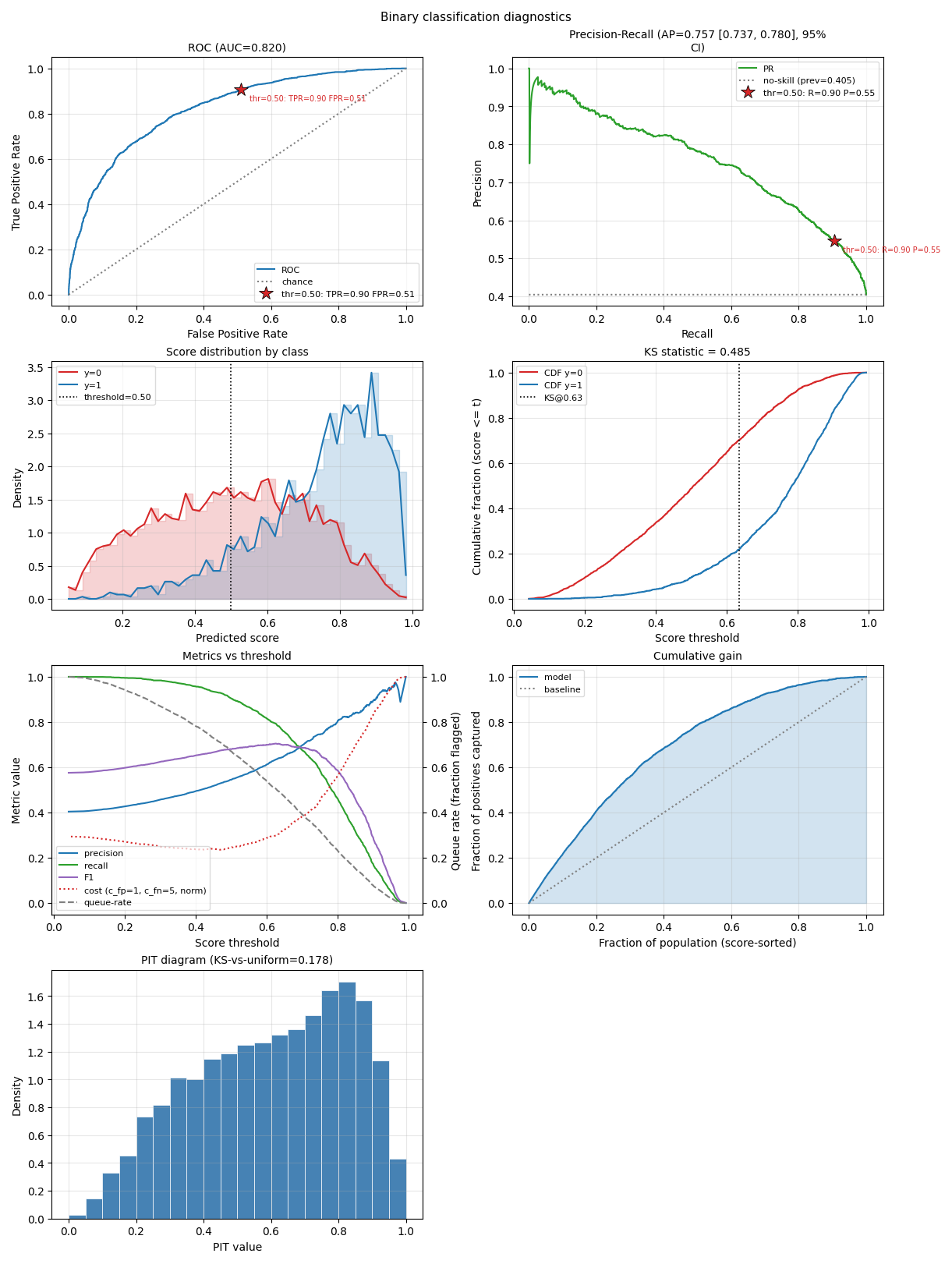
| Binary | ROC PR SCORE_DIST KS THRESHOLD GAIN PIT (binary_panels) |
| Multiclass | CONFUSION CONFUSION_MARGINS CONFUSED_PAIRS PR_F1 ROC CALIB_GRID PROB_DIST TOP_K_ACC (multiclass_panels) |
| Multilabel | PR_F1 CALIB_GRID COOCCURRENCE CARDINALITY JACCARD_DIST THRESHOLD_SWEEP (multilabel_panels) |
| LTR | NDCG_K NDCG_DIST NDCG_BY_QSIZE LIFT MRR_DIST SCORE_BY_REL (ltr_panels) |
| Quantile | RELIABILITY COVERAGE PINBALL_BY_ALPHA INTERVAL_BAND WIDTH_DIST PIT_HIST QUANTILE_RELIABILITY PINBALL_DECOMP QUANTILE_CROSSING FAN_CHART (quantile_panels) |
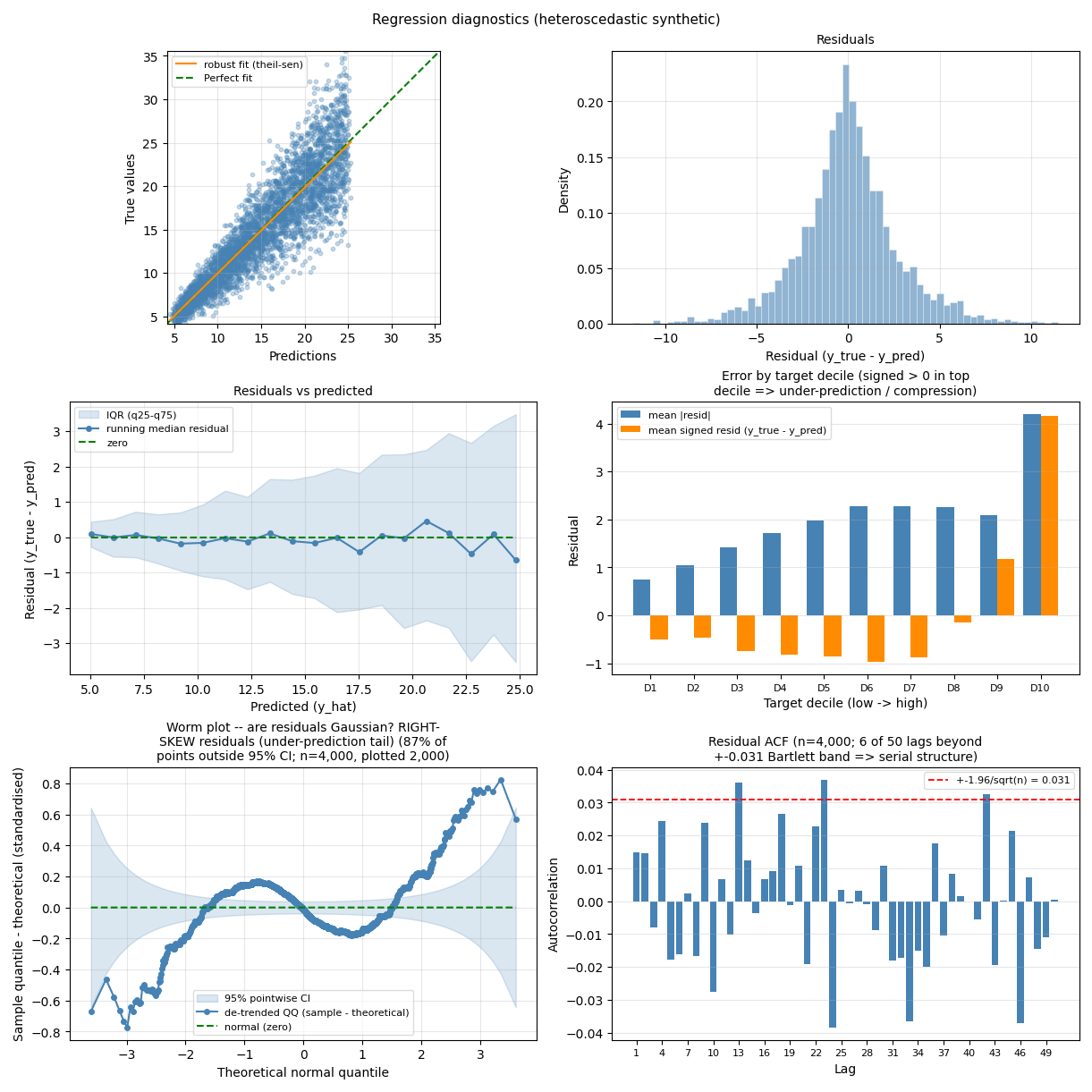
| Regression | SCATTER RESID_HIST RESID_VS_PRED ERR_BY_DECILE WORM RESID_ACF (regression_panels) |
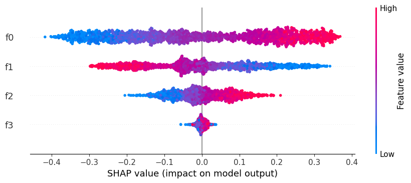
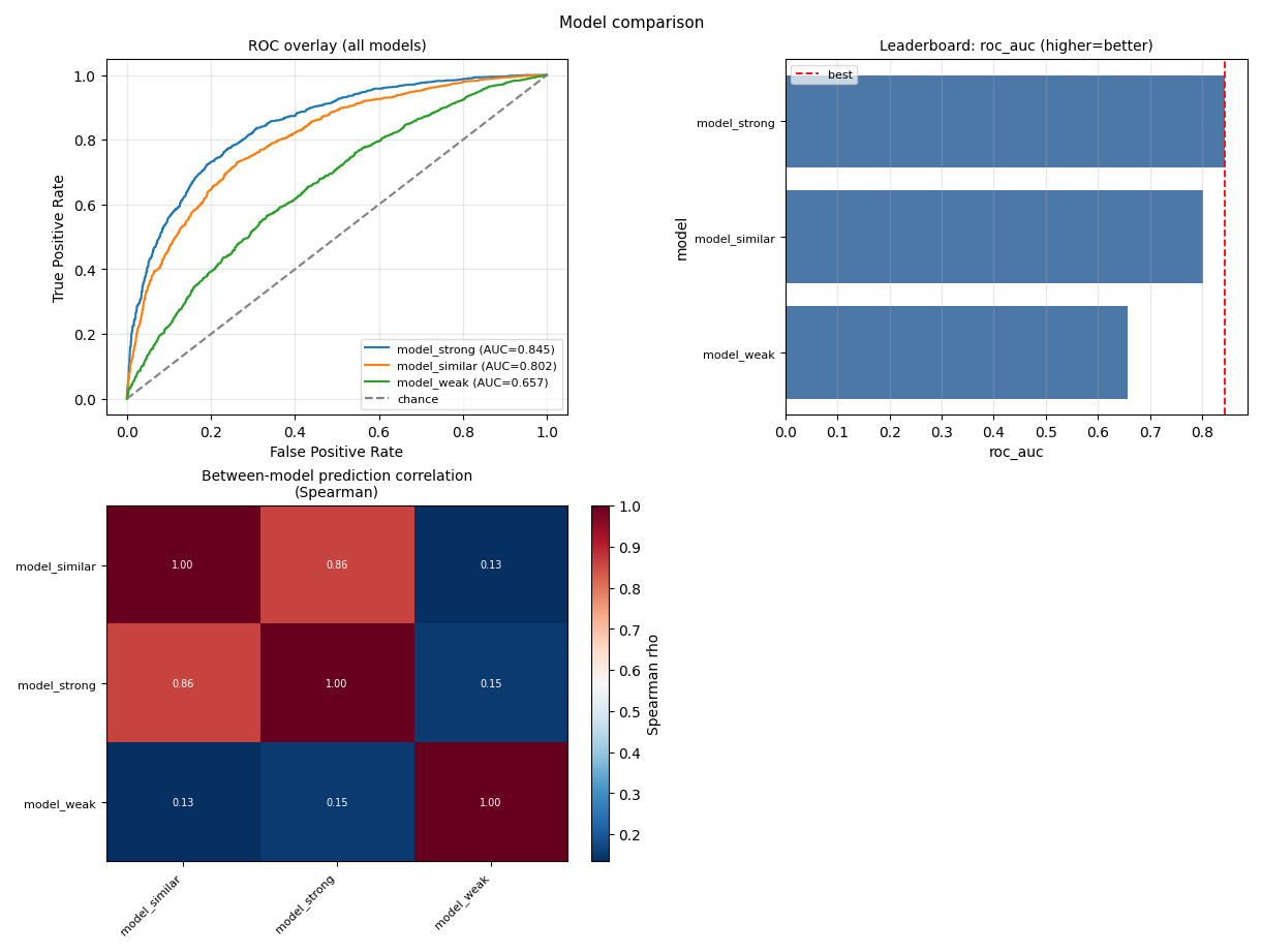
A sample of the rendered panels (full gallery: docs/gallery, regenerated with python scripts/render_gallery.py):
Binary classification (ROC PR SCORE_DIST KS THRESHOLD GAIN PIT) | Regression (scatter, residuals, error-by-decile, worm, ACF) |
 |  |
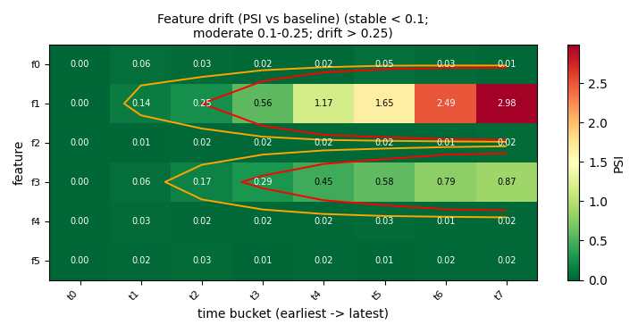
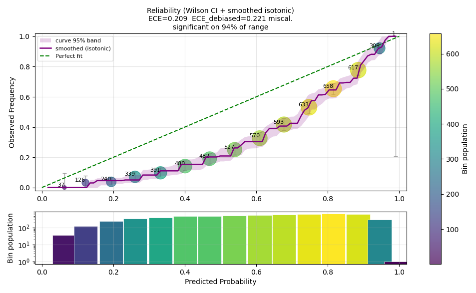
| PSI drift heatmap (feature × time) | Calibration reliability (Venn-Abers / isotonic / Platt / beta) |
 |  |
| SHAP beeswarm | Model comparison across metrics |
 |  |
New diagnostics this brings. Binary classification gained the full curve set it previously lacked (ROC / PR / score-distribution / KS / threshold-sweep / cumulative-gain / PIT). Beyond the per-task panels the suite also renders, when charts are being saved: a target/prediction distribution overlay per split (incl. OOF-vs-test), a tree-guided weak-segment error heatmap, error-bias-per-feature (OVER/UNDER/MAJORITY tails), a worst-K errors table with the same points red-highlighted on the scatter, a PSI drift heatmap (feature × time, 0.10/0.25 triage), adversarial validation (train-vs-test/val LightGBM AUC + drifting-feature bars — "will my CV transfer?"), residual / metric over time, per-model training curves (train vs val metric per boosting iteration with the early-stop point marked), and the quantile reliability / coverage / pinball-by-alpha / PIT / crossing diagnostics including a CORP pinball decomposition.
Large-n behavior. The charts stay cheap on multi-million-row frames with no
pre-subsampling: the regression scatter switches to a log-density hexbin/hist2d
above 50k points (raw scatter with an extremes-preserving subsample below it, so
the MaxError point is always drawn); plotly scatters use Scattergl (WebGL)
above 10k and decimate above 50k; histograms are numpy-prebinned at ≥50k
(2M raw values → ~37MB HTML drops to ~14KB); curves are vertex-decimated to
~2000 points; violins/KDE subsample to 5000; PSI / overlays / over-time panels
are aggregate-first (one O(n) pass per feature).
Output DSL. ReportingConfig.plot_outputs is a backend×format DSL, default
"plotly[html] + matplotlib[png]" — interactive HTML for sharing plus a static
PNG from matplotlib (plotly PNG via kaleido spends ~12-15s/figure on a Chromium
reload, so the fast matplotlib path is the default; use "plotly[html,png]" to
force kaleido). Grammar: <backend>[<fmt>,...] + <backend>[<fmt>,...].
Panel templates are space-separated token strings validated at config
construction against each chart module's allowed-token set, so a typo fails
before training starts. Set any subset (or "" to skip a task's panels).
Key knobs: binary_panels / multiclass_panels / multilabel_panels /
ltr_panels / quantile_panels / regression_panels (panel templates),
regression_scatter_sample_size (5000), calibration_binning
(auto/uniform/quantile), reliability_show_ci (Wilson CI band, on),
training_curves (on), keep_figure_handles (retain pure-data FigureSpecs
in metrics["figure_specs"] for programmatic re-render; chart paths are always
in metrics["charts"]).
Discovery. from mlframe.reporting import describe_available_panels; describe_available_panels() prints every token per task type with a one-line
description (and returns the same mapping for programmatic use).
Caching strategy
The training suite runs two caching layers with different key strategies, because the lifetime of the cached value, the cost of computing the key, and the failure mode of a stale hit differ between them.
Layer 1: _PRE_PIPELINE_CACHE (content-keyed). Caches the output of
(SimpleImputer + StandardScaler + feature selectors).fit_transform(train_df, val_df)
so consecutive models in one suite call that share the same pre-pipeline structure
reuse the fitted transforms. Keys come from content fingerprints of train_df,
val_df, and the target array, the pipeline signature, the target name, and
optionally sample weights. Consecutive lookups see the same Python objects (same id()) but the value
differs across targets, so id-keying would alias entries and content-keying is the
only safe option. The hash cost is amortised across the pre-pipeline fit a hit skips.
Layer 2: FeatureCache.InMemoryKey (id-keyed). Caches per-column intermediate
stats (MRMR scores, target-encoder folds, RFECV ranks) within a single suite call.
Keys are tuples of (session_id, id(train_df), id(train_idx), column, params_canonical_hash, provider_signature). id() is safe here because the suite
holds strong references to train_df and train_idx for its whole lifetime, and the
per-call session_id prevents cross-call collisions. These hits land in inner
per-column loops where a content hash per lookup would dominate the work the cache is
meant to skip. Cross-session reuse is provided separately by a content-keyed DiskKey.
In short: layer 1 spans model boundaries inside one suite call (content-keying
mandatory because intermediate frames are deleted between fits and id()s recycle);
layer 2 spans only inner-loop boundaries where suite-level strong references keep
id() stable, so id-keying is cheap and safe.
Design notes
- Modular, opt-in extras. The core install pulls only the lightweight stack;
heavy dependencies (CatBoost, PyTorch, MLflow, SHAP, plotly) are extras and are
lazy-imported at call site, so nothing fails on
import mlframe. - Polars-native where it matters. Tree models that accept Arrow-backed frames
(CatBoost, HGB, XGBoost) skip the polars-to-pandas round-trip; non-native models
get a zero-copy Arrow view via
pyarrow.Table.to_pandas(zero_copy_only=True). - scikit-learn version pinning. A dedicated sklearn-matrix CI workflow tests the composite-target wrapper surface against scikit-learn 1.6 through 1.8 on every PR, catching attribute-delegation breakage before users hit it.
- Fuzz-tested. Roughly 150 pairwise and 400 three-wise (IPOG-covering) parameter combos run per release. Combo regressions become permanent sensors so they do not recur.
Roadmap
Operations that do not fit the current pipeline-slot abstractions are parked here pending a refactor:
- Row-wise transformations (per-sample normalisation).
Normalizerprojects each sample onto a unit hypersphere, which suits text/embedding similarity but silently breaks tree models that rely on absolute feature magnitudes. A dedicatedrow_transformpipeline slot is planned so row-wise operations have an unambiguous home that cannot be confused with column scalers.
Testing
pytest                                    # full suite
pytest -m fast                            # representative subset (<15s)
pytest -m "not slow and not gpu"          # CI default
pytest --cov=src/mlframe --cov-report=html
Markers: slow, integration, gpu, multigpu, benchmark, windows_only,
linux_only, fast.
Environment variables
Every environment variable read anywhere in src/mlframe/ via os.environ.get(...) / os.getenv(...), generated from the source (name, first read site, and its literal default if one is passed inline). This is a mechanically-generated inventory, not a hand-written guide -- it documents that a var is read and its default, not why it exists or what it tunes; see the linked file for that.
Contributing
Pull requests are welcome. Code style is black + ruff with a line length of 160.
Every new feature ships with a unit test, a quantitative business-value test, a
representative @pytest.mark.fast subset, and a cProfile hotspot check. See
CONTRIBUTING.md for the full development workflow, test bar, and
the fuzz / combo test philosophy.
License
MIT, see LICENSE.